
MR.RGM fits Bayesian reciprocal graphical models for
instrumental-variable (IV) analysis of several responses at once. From
instruments X, responses Y and optional
measured covariates U, RGM() estimates the
direct causal effects among the responses, which may form directed
cycles, the effects of the instruments, and the structure of unmeasured
confounding among the responses, with a posterior inclusion probability
for every edge and every confounding link. NetworkMotif()
gives the posterior probability of any set of edges, such as a feedback
loop. The package is named after its first application, Mendelian
randomization (MR), in which genetic variants are the instruments, but
the model applies to instrumental variables in general.
RGM accommodates both individual-level data and two types of summary-level data, making it adaptable to various data availability scenarios. In addition, RGM optionally allows the inclusion of observed covariates, enabling adjustment for measured confounders when such information is available. Covariates can be incorporated using either individual-level data or corresponding summary-level matrices.
The outputs of RGM() include the estimated causal
effects and their inclusion probabilities, the instrument and covariate
effects, the error covariance and, under the "SSSL" error
model, the inclusion probabilities of its off-diagonal entries, which
describe unmeasured confounding between pairs of responses.
RGM() also returns diagnostics of weak instruments, weak
identification and convergence, with a warning when one of them signals
a problem.
You can install the released version of MR.RGM from CRAN with:
install.packages("MR.RGM")You can install version 0.1.3, the version used for the analyses in
reproducibility/, from GitHub with:
    # install.packages("remotes")
    remotes::install_github("bitansa/MR.RGM")
The model has no intercept and the "SSSL" error model
assumes responses on roughly unit scale, so center and scale real data
before fitting (see ?RGM).
The input can be individual-level data (X,
Y, optionally U), the second-moment matrices
of one sample (Syy, Syx, Sxx, and
Syu, Sxu, Suu for covariates), or
marginal instrument–response regressions (Sxx,
Beta, SigmaHat). The last input does not
contain the covariances between the responses, which are reconstructed
under independent errors: it therefore requires
SigmaStarModel = "diagonal", no covariates, an instrument
that affects only one response for every response, and uncorrelated
instruments, and SigmaHat holds the residual sums of
squares divided by n. Unmeasured confounding can be modeled
only from individual-level data or the second-moment matrices.
The model applies to instrumental variables in general, not only to genetic instruments; in the accompanying methods paper the two versions are called IV-RGM and IV-RGM+.
The instrument–response map D (a binary
p x k matrix, D[i, j] = 1 if instrument
j may affect response i) decides which version
is fitted:
D with zeros, the usual case:
each instrument assigned to its own response, e.g. a cis-eQTL to its
gene): entries of B with D = 0 are fixed at
zero and the allowed entries receive a slab prior without selection, so
every allowed instrument stays in the model. The causal effects are
identified through the excluded instruments (rank condition).D all ones): every entry of
B receives a spike-and-slab prior and the map is learned
from the data, which accommodates horizontal pleiotropy. This needs
instruments that explain a non-negligible share of the variance; with
many weak instruments the fit is weakly identified and
RGM() warns.The argument selectB overrides this default
(selectB = TRUE with a partial D selects among
the allowed entries; selectB = FALSE with
D = 1 gives every entry a slab prior). The value used is
stored in fit$settings$selectB.
Once the MR.RGM package is installed load the package.
library("MR.RGM")The examples below use simulated data to illustrate
RGM() with individual-level data, summary-level data and
the alternative error models, and the estimation of the effects among
the responses, of the instruments and, when present, of the covariates.
The last example applies NetworkMotif() to the posterior
draws GammaPst returned by RGM().
# Model: Y = AY + BX + CU + E

# Set seed
set.seed(9154)

# Number of data points
n = 30000

# Number of response variables, instruments, and covariates
p = 5
k = 6
l = 2

# Initialize causal interaction matrix between response variables
A = matrix(sample(c(-0.1, 0.1), p^2, replace = TRUE), p, p)

# Diagonal entries of A matrix will always be 0
diag(A) = 0

# Make the network sparse
A[sample(which(A != 0), length(which(A != 0)) / 2)] = 0

# Create D matrix (Indicator matrix: rows = responses, cols = instruments)
D = matrix(0, nrow = p, ncol = k)

# Manually assign values to D matrix
D[1, 1:2] = 1
D[2, 3]   = 1
D[3, 4]   = 1
D[4, 5]   = 1
D[5, 6]   = 1

# Initialize B matrix (instrument effects)
B = matrix(0, p, k)
for (i in 1:p) {
  for (j in 1:k) {
    if (D[i, j] == 1) {
      B[i, j] = 1
    }
  }
}

# Generate covariate data matrix U (n x l)
U = matrix(rnorm(n * l), nrow = n, ncol = l)

# Initialize C matrix (covariate effects)
C = matrix(0, p, l)
C[sample(length(C), size = ceiling(length(C) / 2))] = 1

# Create a full (non-diagonal) positive definite error covariance matrix Sigma
R = matrix(rnorm(p * p), p, p)
Sigma = crossprod(R)                 # SPD

# Compute (I - A)^{-1}
Mult_Mat = solve(diag(p) - A)

# Variance of Y
Variance = Mult_Mat %*% Sigma %*% t(Mult_Mat)

# Generate instrument data matrix X
X = matrix(rnorm(n * k), nrow = n, ncol = k)

# Initialize response data matrix Y
Y = matrix(0, nrow = n, ncol = p)

# Generate response data
for (i in 1:n) {
  mu_i = Mult_Mat %*% (B %*% X[i, ] + C %*% U[i, ])
  Y[i, ] = as.numeric(mu_i + t(chol(Variance)) %*% rnorm(p))   # multivariate normal draw
}

# The model has no intercept and the SSSL prior assumes responses on unit scale:
# center and scale every column (the estimates are then on the standardized scale)
X = scale(X); Y = scale(Y); U = scale(U)

# Print true causal interaction matrices
A
#>      [,1] [,2] [,3] [,4] [,5]
#> [1,]  0.0 -0.1  0.0  0.0  0.1
#> [2,]  0.1  0.0 -0.1  0.1  0.1
#> [3,]  0.0 -0.1  0.0  0.0  0.1
#> [4,]  0.0 -0.1  0.0  0.0  0.0
#> [5,]  0.0  0.1  0.0  0.0  0.0
B
#>      [,1] [,2] [,3] [,4] [,5] [,6]
#> [1,]    1    1    0    0    0    0
#> [2,]    0    0    1    0    0    0
#> [3,]    0    0    0    1    0    0
#> [4,]    0    0    0    0    1    0
#> [5,]    0    0    0    0    0    1
C
#>      [,1] [,2]
#> [1,]    1    0
#> [2,]    1    0
#> [3,]    0    1
#> [4,]    0    0
#> [5,]    1    1
We will now apply RGM using individual-level data and summary-level data to demonstrate its functionality.
# ---------------------------------------------------------
# Apply RGM on individual-level data with covariates (Spike and Slab prior)
# Model: Y = AY + BX + CU + E

Output1 = RGM(
  X = X, Y = Y, U = U,
  D = D, nIter = 50000, nBurnin = 10000, Thin = 10,
  prior = "Spike and Slab",
  SigmaStarModel = "IW"
)

# ---------------------------------------------------------
# Compute summary-level quantities (including covariates)
Syy = crossprod(Y) / n        # t(Y) %*% Y / n
Syx = t(Y) %*% X / n
Sxx = crossprod(X) / n        # t(X) %*% X / n

Syu = t(Y) %*% U / n
Sxu = t(X) %*% U / n
Suu = crossprod(U) / n        # t(U) %*% U / n

# Apply RGM on summary-level data with covariates (Spike-and-Slab prior)
Output2 = RGM(
  Syy = Syy, Syx = Syx, Sxx = Sxx,
  Syu = Syu, Sxu = Sxu, Suu = Suu,
  D = D, n = n, nIter = 50000, nBurnin = 10000, Thin = 10,
  prior = "Spike and Slab",
  SigmaStarModel = "SSSL"
)
We get the estimated causal interaction matrix between response variables in the following way:
Output1$AEst
#>              [,1]        [,2]         [,3]         [,4]        [,5]
#> [1,]  0.000000000 -0.08576742 -0.000892405  0.008341425 0.079103702
#> [2,]  0.126641588  0.00000000 -0.077143750  0.107618630 0.111005823
#> [3,]  0.002795267 -0.10188060  0.000000000 -0.001605146 0.121469458
#> [4,] -0.001997341 -0.08517978 -0.005094947  0.000000000 0.001624467
#> [5,]  0.001391380  0.09080841 -0.006854622  0.001749397 0.000000000
Output2$AEst
#>              [,1]        [,2]          [,3]         [,4]        [,5]
#> [1,]  0.000000000 -0.08609198 -0.0006708842  0.006892759 0.080046085
#> [2,]  0.125502480  0.00000000 -0.0765547106  0.108836415 0.110620750
#> [3,]  0.003255845 -0.10064567  0.0000000000 -0.002832670 0.121947656
#> [4,] -0.001482171 -0.08546426 -0.0047973763  0.000000000 0.000834903
#> [5,]  0.002093526  0.09134678 -0.0066718731  0.001787908 0.000000000
We get the estimated causal network structure between the response variables in the following way:
Output1$zAEst
#>      [,1] [,2] [,3] [,4] [,5]
#> [1,]    0    1    0    0    1
#> [2,]    1    0    1    1    1
#> [3,]    0    1    0    0    1
#> [4,]    0    1    0    0    0
#> [5,]    0    1    0    0    0
Output2$zAEst
#>      [,1] [,2] [,3] [,4] [,5]
#> [1,]    0    1    0    0    1
#> [2,]    1    0    1    1    1
#> [3,]    0    1    0    0    1
#> [4,]    0    1    0    0    0
#> [5,]    0    1    0    0    0
We get the estimated causal interaction matrix between the response and the instrument variables from the outputs in the following way:
Output1$BEst
#>          [,1]     [,2]      [,3]      [,4]      [,5]     [,6]
#> [1,] 0.355555 0.368797 0.0000000 0.0000000 0.0000000 0.000000
#> [2,] 0.000000 0.000000 0.4589062 0.0000000 0.0000000 0.000000
#> [3,] 0.000000 0.000000 0.0000000 0.4995741 0.0000000 0.000000
#> [4,] 0.000000 0.000000 0.0000000 0.0000000 0.4280438 0.000000
#> [5,] 0.000000 0.000000 0.0000000 0.0000000 0.0000000 0.413484
Output2$BEst
#>           [,1]      [,2]      [,3]      [,4]      [,5]      [,6]
#> [1,] 0.3556305 0.3688838 0.0000000 0.0000000 0.0000000 0.0000000
#> [2,] 0.0000000 0.0000000 0.4583299 0.0000000 0.0000000 0.0000000
#> [3,] 0.0000000 0.0000000 0.0000000 0.4993608 0.0000000 0.0000000
#> [4,] 0.0000000 0.0000000 0.0000000 0.0000000 0.4286899 0.0000000
#> [5,] 0.0000000 0.0000000 0.0000000 0.0000000 0.0000000 0.4134184
With a known instrument map D, as here, the graph
between the instruments and the responses is fixed and
zBEst equals D; it is estimated only when the
instrument effects are selected (selectB = TRUE):
Output1$zBEst
#>      [,1] [,2] [,3] [,4] [,5] [,6]
#> [1,]    1    1    0    0    0    0
#> [2,]    0    0    1    0    0    0
#> [3,]    0    0    0    1    0    0
#> [4,]    0    0    0    0    1    0
#> [5,]    0    0    0    0    0    1
Output2$zBEst
#>      [,1] [,2] [,3] [,4] [,5] [,6]
#> [1,]    1    1    0    0    0    0
#> [2,]    0    0    1    0    0    0
#> [3,]    0    0    0    1    0    0
#> [4,]    0    0    0    0    1    0
#> [5,]    0    0    0    0    0    1
The estimated causal effects of covariates on the response variables are obtained as follows:
Output1$CEst
#>              [,1]         [,2]
#> [1,]  0.374731037  0.006568381
#> [2,]  0.460967976 -0.007272777
#> [3,]  0.001791698  0.503900967
#> [4,] -0.012180539  0.005039516
#> [5,]  0.404093750  0.414730125
Output2$CEst
#>               [,1]         [,2]
#> [1,]  0.3744263542  0.005863437
#> [2,]  0.4614858157 -0.007309617
#> [3,]  0.0007802109  0.503666847
#> [4,] -0.0119836335  0.005161626
#> [5,]  0.4034761217  0.414499628
We can plot the log-likelihoods from the outputs in the following way:
plot(Output1$LLPst, type = 'l', xlab = "Iterations", ylab = "Log-likelihood")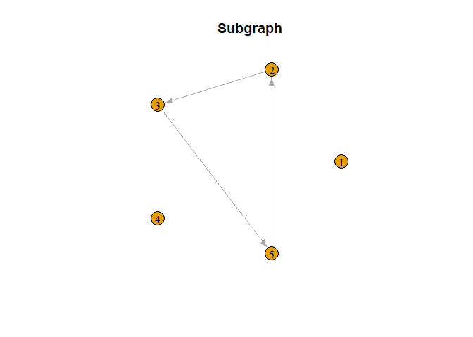
plot(Output2$LLPst, type = 'l', xlab = "Iterations", ylab = "Log-likelihood")
Next, we present the implementation of the NetworkMotif function. We begin by defining a motif (subgraph) among the response variables. Subsequently, we collect GammaPst arrays from various outputs and proceed to execute NetworkMotif based on these arrays.
# Define a function to create smaller arrowheads
smaller_arrowheads <- function(graph) {
  igraph::E(graph)$arrow.size = 0.60  # Adjust the arrow size value as needed
  return(graph)
}

# Define a motif (subgraph) among the responses
Gamma = matrix(0, nrow = p, ncol = p)
Gamma[5, 2] = Gamma[3, 5] = Gamma[2, 3] = 1

# Plot the motif
plot(smaller_arrowheads(igraph::graph_from_adjacency_matrix(t(Gamma),   # A[i, j]: effect of Y_j on Y_i
       mode = "directed")), layout = igraph::layout_in_circle,
          main = "Subgraph")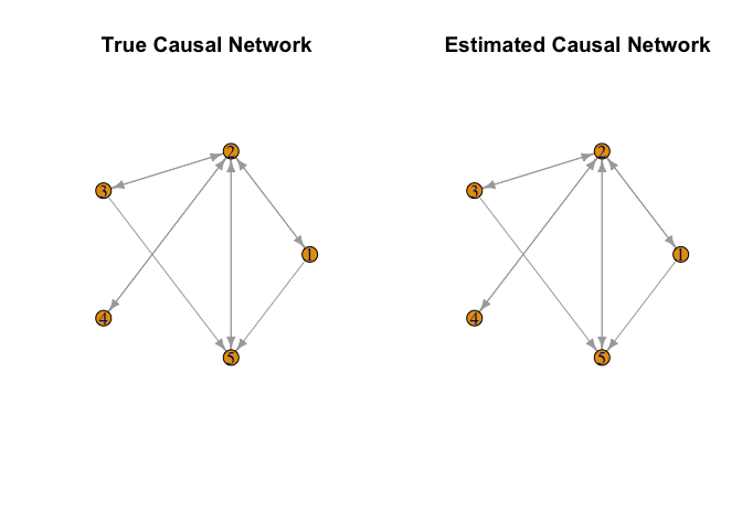
# Store the GammaPst arrays from outputs
GammaPst1 = Output1$GammaPst
GammaPst2 = Output2$GammaPst

# Get the posterior probabilities of Gamma with these GammaPst matrices
NetworkMotif(Gamma = Gamma, GammaPst = GammaPst1)
#> [1] 0.34775
NetworkMotif(Gamma = Gamma, GammaPst = GammaPst2)
#> [1] 0.3635In real-world scenarios, it is common to encounter a large number of instrumental variables (IVs), each explaining only a small proportion of the trait variance. The following simulation setting reflects this:
compact_X: By combining
the top PCs from each response variable, we form a condensed matrix
compact_X. This matrix aggregates the instrumental
variables into a more manageable form, facilitating a more efficient
analysis.compact_X, we calculate new summary level data
(Sxx_compact and Syx_compact) for the RGM
function application. This approach provides a more realistic
representation of the instrumental variables’ effects in scenarios with
many IVs explaining only a small proportion of the variance.The R code for this setting:
# (No covariates in this example) Model: Y = AY + BX + E

# Set seed for reproducibility
set.seed(9154)

# Number of data points
n = 10000

# Number of response variables
p = 5

# Number of SNPs per response variable
num_snps_per_y = 100

# Total number of SNPs
k = num_snps_per_y * p

# Initialize causal interaction matrix between response variables
A = matrix(sample(c(-0.1, 0.1), p^2, replace = TRUE), p, p)
diag(A) = 0
A[sample(which(A != 0), length(which(A != 0)) / 2)] = 0

# Create D matrix (Indicator matrix where each row corresponds to a response variable
# and each column corresponds to an instrument variable)
D = matrix(0, nrow = p, ncol = k)

# Assign values to D matrix using a loop
for (run in 1:p) {

  D[run, ((run - 1) * num_snps_per_y + 1) : (run * num_snps_per_y)] = 1

}

# Initialize B matrix
B = matrix(0, p, k)  # Initialize B matrix with zeros

# Calculate B matrix based on D matrix
for (i in 1:p) {
   for (j in 1:k) {
     if (D[i, j] == 1) {
       B[i, j] = 1  # Set B[i, j] to 1 if D[i, j] is 1
     }
   }
 }

# Calculate Variance-Covariance matrix
# Error variance model used to generate Y (diagonal => independent errors across responses)
Sigma = diag(p)
Mult_Mat = solve(diag(p) - A)
Variance = Mult_Mat %*% Sigma %*% t(Mult_Mat)

# Generate instrument data matrix (X)
X = matrix(rnorm(n * k, 0, 1), nrow = n, ncol = k)

# Initialize response data matrix (Y)
Y = matrix(0, nrow = n, ncol = p)

# Generate response data matrix based on instrument data matrix
for (i in 1:n) {
    Y[i, ] = as.numeric(Mult_Mat %*% B %*% X[i, ] + t(chol(Variance)) %*% rnorm(p))
}

# Center and scale the columns (the model has no intercept)
X = scale(X); Y = scale(Y)

# Calculate summary level data
Syy = t(Y) %*% Y / n
Syx = t(Y) %*% X / n
Sxx = t(X) %*% X / n

# PCA-based IV compression:
# mimic many weak SNP instruments per response; keep top PCs to reduce dimension
# Perform PCA for each response variable to get top 20 PCs
top_snps_list = list()
for (i in 1:p) {
    X_sub = X[, (num_snps_per_y * (i - 1) + 1):(num_snps_per_y * i)]
    pca = prcomp(X_sub, center = TRUE, scale. = TRUE)
    top_20_pcs = pca$x[, 1:20]
    top_snps_list[[i]] = top_20_pcs
}

# Combine the top PCs from all response variables
compact_X = do.call(cbind, top_snps_list)

# Calculate summary level data based on compact_X
Sxx_compact = t(compact_X) %*% compact_X / n
Syx_compact = t(Y) %*% compact_X / n

# Create D_New
D_New = matrix(0, nrow = p, ncol = 20 * p)

# Assign values to D matrix using a loop
for (run in 1:p) {

  D_New[run, ((run - 1) * 20 + 1) : (run * 20)] = 1

}

# Apply RGM on summary-level data (Spike-and-Slab prior)
# Since errors were generated independently (Sigma diagonal), set SigmaStarModel = "diagonal"
Output = RGM(Syy = Syy, Syx = Syx_compact, Sxx = Sxx_compact, D = D_New, n = n, prior = "Spike and Slab", SigmaStarModel = "diagonal")

# Print estimated causal interaction matrices
Output$AEst
#>              [,1]        [,2]         [,3]         [,4]       [,5]
#> [1,]  0.000000000 -0.10632215  0.012826398  0.002426187 0.09177666
#> [2,]  0.108236029  0.00000000 -0.098563505  0.087864598 0.10473073
#> [3,] -0.003594494 -0.11229548  0.000000000 -0.007342171 0.10626710
#> [4,] -0.002508607 -0.08843764  0.011327468  0.000000000 0.01096636
#> [5,] -0.001073286  0.11100250 -0.003778593 -0.010798651 0.00000000
Output$zAEst
#>      [,1] [,2] [,3] [,4] [,5]
#> [1,]    0    1    0    0    1
#> [2,]    1    0    1    1    1
#> [3,]    0    1    0    0    1
#> [4,]    0    1    0    0    0
#> [5,]    0    1    0    0    0

# Create a layout for multiple plots
par(mfrow = c(1, 2))

smaller_arrowheads <- function(graph) {
  igraph::E(graph)$arrow.size <- 0.6
  graph
}

# Plot the true causal network
plot(smaller_arrowheads(igraph::graph_from_adjacency_matrix(t((A != 0) * 1), mode = "directed")),
     layout = igraph::layout_in_circle, main = "True Causal Network")

# Plot the estimated causal network
plot(Output$Graph, main = "Estimated Causal Network")
Conclusion
In this setting, with many instruments each explaining a small fraction of the variance of a response, the principal components of the instruments give a smaller set of instruments that retains their joint effect on each response, and MR.RGM recovers the causal network. The same approach applies to other settings with many weak or correlated instruments.
The scripts that reproduce every simulation, table and figure of the
accompanying methods paper, with instructions, are in reproducibility/.
The preprocessed OneK1K B-cell data used in its application are archived
on Zenodo, https://doi.org/10.5281/zenodo.18489687, and the result
files of the paper, from which the scripts regenerate every table and
figure, at https://doi.org/10.5281/zenodo.24043120. To cite the
package, run citation("MR.RGM").
Bitan Sarkar and Yang Ni. “MR.RGM: an R package for fitting Bayesian multivariate bidirectional Mendelian randomization networks.” Bioinformatics 41 (4), btaf130, 2025. https://doi.org/10.1093/bioinformatics/btaf130
Yang Ni, Yuan Ji and Peter Müller. “Reciprocal Graphical Models for Integrative Gene Regulatory Network Analysis.” Bayesian Anal. 13 (4) 1095 - 1110, December 2018. https://doi.org/10.1214/17-BA1087