cforecast is an R package for interpretable scenario analysis in reduced-form vector autoregressive (VAR) models. Using a Kalman filtering and smoothing framework, it generates conditional forecasts under path restrictions on selected variables and provides tools to explain how these restrictions shape forecast outcomes. The package decomposes conditional forecasts into variable-specific contributions, extracts observation weights, and computes measures of overall and marginal variable importance. These diagnostics reveal which assumptions drive forecast revisions and quantify the model’s sensitivity to alternative scenario paths. Because the framework is structurally agnostic, it is well suited for policy analysis, stress testing, and macro-financial applications where transparency and interpretability are essential.
The current version introduces support for the KFAS
backend for state-space filtering and smoothing
(package = "KFAS"). This backend is more robust in the
presence of singular or near-singular forecast error variance matrices,
where the default FKF implementation may fail, at the cost
of increased computation time.
The example below replicates an empirical experiment from:
Caspi, I., & Ginker, T. (2026). What Drives the Scenario? Interpreting Conditional Forecasts in Reduced-Form VARs.
The illustration demonstrates the workflow for scenario design, conditional forecasting, and forecast attribution.
Install the development version from GitHub:
# install.packages("devtools")
devtools::install_github("timginker/cforecast")This section demonstrates how the conditional forecasting tools in
cforecast can be used to:
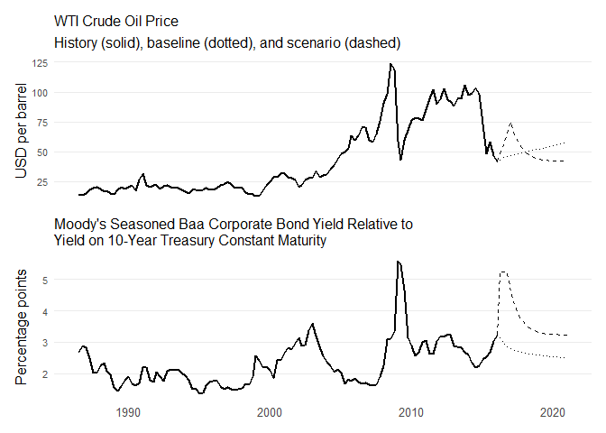
We consider a stylized policy scenario combining:
Such scenarios are typical in monetary policy and macro-financial stress-testing applications.
We use U.S. quarterly macroeconomic data (1986Q2–2015Q4) from
FRED.
The dataset includes the following series:
The VAR includes five variables:
Below, we estimate a reduced-form VAR(2) with a constant term and compute a 20-quarter baseline (unconditional) forecast.
suppressPackageStartupMessages({
library(cforecast)
library(tidyverse)
library(vars)
library(lubridate)
library(scales)
library(patchwork)
})

# ---------- 1. Data --------------------------------------------------
data(fred_macro)         # GDPC1, PCEPILFE Q/Q %; FEDFUNDS, BAA10YM level; DCOILWTICO Q/Q %
data(DCOILWTICO_level)   # WTI level (for plotting only)

VAR_NAMES <- c("GDPC1", "PCEPILFE", "FEDFUNDS", "BAA10YM", "DCOILWTICO")
LABELS <- c(
  GDPC1      = "Real GDP growth",
  PCEPILFE   = "Core PCE inflation",
  FEDFUNDS   = "Federal funds rate",
  BAA10YM    = "Baa-10Y credit spread",
  DCOILWTICO = "WTI crude oil price"
)

# Estimation sample: 1986Q2 .. 2015Q4 (paper sample, T+1 = 2016Q1)
sample_data <- subset(fred_macro, date <= as.Date("2015-12-31"))
y_mat       <- as.matrix(sample_data[, VAR_NAMES])

T_hist     <- nrow(y_mat)
last_date  <- max(sample_data$date)

# ---------- 2. VAR estimation: VAR(p) with constant, p chosen by BIC -
sel <- VARselect(y_mat, lag.max = 8, type = "const")
p_bic <- sel$selection["SC(n)"]
fit <- VAR(y_mat, p = p_bic, type = "const")
# Baseline forecast
unc_fc <- predict(fit, n.ahead = 20)We construct a two-variable conditioning path affecting:
The scenario is designed as follows:
This structure mimics a temporary macro-financial stress episode with persistent but fading effects.
The following plot creates the scenario and plots it:
H              <- 20
forecast_dates <- seq(as.Date("2016-03-31"), by = "3 months", length.out = H)

baa_idx <- which(VAR_NAMES == "BAA10YM")
oil_idx <- which(VAR_NAMES == "DCOILWTICO")
pce_idx <- which(VAR_NAMES == "PCEPILFE")

baa_base <- unc_fc$fcst[["BAA10YM"]][, "fcst"]
oil_base <- unc_fc$fcst[["DCOILWTICO"]][, "fcst"]   # Q/Q %
pce_base <- unc_fc$fcst[["PCEPILFE"]][, "fcst"]

# Scenario (Section 3 of paper):
#   * Credit spread: ~200bp widening, decays toward ~3.2
#   * WTI: rises to peak ~$75 in 2016Q4, then mean-reverts to ~$40-43
baa_scen <- 3.2 + 2.0 * exp(-0.5 * (0:(H - 1)))

last_oil_level <- subset(DCOILWTICO_level,
                         date == as.Date("2015-12-31"))$DCOILWTICO
oil_target_levels <- c(48, 58, 70, 75, 72, 62, 50, 44,
                       42, 40, 41, 42, 42, 41, 42, 43, 42, 41, 43, 42)
oil_scen <- diff(c(last_oil_level, oil_target_levels)) /
              c(last_oil_level, oil_target_levels[-H]) * 100  # Q/Q %

# Build the level path implied by the unconditional baseline (plotting)
oil_base_levels <- numeric(H); prev <- last_oil_level
for (i in seq_len(H)) {
  oil_base_levels[i] <- prev * (1 + oil_base[i] / 100)
  prev <- oil_base_levels[i]
}


# Table 01: scenario inputs (Figure 1) --------------------------------
hist_wti <- subset(DCOILWTICO_level,
                   date <= as.Date("2015-12-31") & date >= as.Date("1986-06-30"))

t01_wti <- bind_rows(
  hist_wti %>% transmute(date, series = "WTI", type = "Historical",
                         value = DCOILWTICO),
  tibble(date = forecast_dates, series = "WTI",
         type = "Baseline (unconditional)", value = oil_base_levels),
  tibble(date = forecast_dates, series = "WTI",
         type = "Scenario", value = oil_target_levels)
)
t01_baa <- bind_rows(
  sample_data %>% transmute(date, series = "BAA10YM",
                            type = "Historical", value = BAA10YM),
  tibble(date = forecast_dates, series = "BAA10YM",
         type = "Baseline (unconditional)", value = baa_base),
  tibble(date = forecast_dates, series = "BAA10YM",
         type = "Scenario", value = baa_scen)
)

wti_df <- bind_rows(
  hist_wti %>% transmute(date, value = DCOILWTICO, type = "Historical"),
  tibble(date = forecast_dates, value = oil_base_levels,
         type = "Baseline (unconditional)"),
  tibble(date = forecast_dates, value = oil_target_levels,
         type = "Scenario"),
  tibble(date = last_date,
         value = subset(DCOILWTICO_level, date == last_date)$DCOILWTICO,
         type = "Baseline (unconditional)"),
  tibble(date = last_date,
         value = subset(DCOILWTICO_level, date == last_date)$DCOILWTICO,
         type = "Scenario")
)


# =====================================================================
# FIGURE STYLING
# =====================================================================
COL <- list(
  navy   = "#1B365D", blue = "#3B5C8A", yellow = "#E8D055",
  gold   = "#D4B43F", gray = "#8B8B8B", beige  = "#C0B392",
  red    = "#C84050"
)
PALETTE_VAR <- c(
  BAA10YM    = COL$navy,
  DCOILWTICO = COL$blue,
  FEDFUNDS   = COL$gray,
  GDPC1      = COL$beige,
  PCEPILFE   = COL$yellow
)

theme_boi <- function(base_size = 11) {
  theme_minimal(base_size = base_size) +
    theme(
      plot.title         = element_text(face = "bold", size = rel(1.0),
                                        hjust = 0, margin = margin(b = 2)),
      plot.subtitle      = element_text(size = rel(0.85), color = "grey25",
                                        hjust = 0, margin = margin(b = 6)),
      panel.grid.major.x = element_blank(),
      panel.grid.minor   = element_blank(),
      panel.grid.major.y = element_line(color = "grey88", linewidth = 0.4),
      axis.title         = element_text(size = rel(0.85)),
      axis.text          = element_text(size = rel(0.85), color = "grey20"),
      axis.ticks.x       = element_line(color = "grey50"),
      axis.ticks.y       = element_blank(),
      axis.line.x        = element_line(color = "grey50"),
      legend.position    = "top",
      legend.title       = element_blank(),
      legend.text        = element_text(size = rel(0.8)),
      legend.key.size    = unit(0.7, "lines"),
      plot.margin        = margin(8, 12, 8, 12)
    )
}

p_wti <- ggplot(wti_df, aes(date, value, linetype = type, group = type)) +
  geom_line(linewidth = 0.55, color = "black") +
  scale_linetype_manual(values = c("Historical" = "solid",
                                   "Baseline (unconditional)" = "dotted",
                                   "Scenario" = "dashed")) +
  scale_y_continuous(breaks = c(25, 50, 75, 100, 125)) +
  scale_x_date(breaks = as.Date(paste0(seq(1990, 2020, 10), "-01-01")),
               date_labels = "%Y") +
  labs(title = "WTI Crude Oil Price",
       x = NULL, y = "USD per barrel") +
  theme_boi() + theme(legend.position = "none")

last_baa <- tail(sample_data$BAA10YM, 1)
baa_df <- bind_rows(
  sample_data %>% transmute(date, value = BAA10YM, type = "Historical"),
  tibble(date = forecast_dates, value = baa_base,
         type = "Baseline (unconditional)"),
  tibble(date = forecast_dates, value = baa_scen, type = "Scenario"),
  tibble(date = last_date, value = last_baa,
         type = "Baseline (unconditional)"),
  tibble(date = last_date, value = last_baa, type = "Scenario")
)

p_baa <- ggplot(baa_df, aes(date, value, linetype = type, group = type)) +
  geom_line(linewidth = 0.55, color = "black") +
  scale_linetype_manual(values = c("Historical" = "solid",
                                   "Baseline (unconditional)" = "dotted",
                                   "Scenario" = "dashed")) +
  scale_y_continuous(breaks = c(2, 3, 4, 5)) +
  scale_x_date(breaks = as.Date(paste0(seq(1990, 2020, 10), "-01-01")),
               date_labels = "%Y") +
  labs(title = paste0("Moody's Seasoned Baa Corporate Bond Yield Relative to\n",
                      "Yield on 10-Year Treasury Constant Maturity"),
       x = NULL, y = "Percentage points") +
  theme_boi() +
  theme(legend.position = "none",
        plot.title = element_text(face = "bold", size = rel(0.92), hjust = 0))

gridExtra::grid.arrange(
  p_wti,
  p_baa,
  ncol = 1,
  heights = c(1, 1.05)
)
We begin by examining overall variable importance in the conditional forecast of core inflation. These measures are computed ex ante, given the conditioning design: the future paths of the corporate credit spread (Moody’s Baa–10Y Treasury spread) and WTI crude oil prices are constrained, while the remaining variables are left unconstrained.
The decomposition therefore quantifies the relative contribution of:
Importantly, this assessment does not require realized future values.
The plot below reports the overall variable importance:
v_imp=variable_importance_stat(fit=fit,
                               cond_var = 4:5,
                               target_var = 2,
                               horizon = 20)

# Visualize variable importance as stacked shares by horizon (normalized to 100%)
plt = ggplot(v_imp$variable_importance,
             aes(x = factor(horizon),
                 y = share,
                 fill = variable)) +
  geom_col(position = "fill", width = 0.75, color = "white", linewidth = 0.2) +
  scale_y_continuous(
    labels = percent_format(accuracy = 1),
    expand = expansion(mult = c(0, 0.02))
  ) +
  scale_fill_viridis_d(option = "cividis", end = 0.9) +
  labs(
    title = "Decomposition of Conditional Core Inflation Forecast",
    subtitle = "Overall variable importance by forecast horizon",
    x = "Forecast horizon (quarters ahead)",
    y = "Share of information (percent)",
    fill = NULL
  ) +
  theme_classic(base_size = 12) +
  theme(
    plot.title = element_text(face = "bold", size = 11),
    plot.subtitle = element_text(size = 10),
    axis.title = element_text(size = 11),
    axis.text  = element_text(size = 10),
    legend.position = "top",
    legend.text = element_text(size = 10),
    legend.key.size = unit(0.35, "cm"),
    axis.line = element_line(linewidth = 0.3),
    axis.ticks = element_line(linewidth = 0.3)
  )

plt 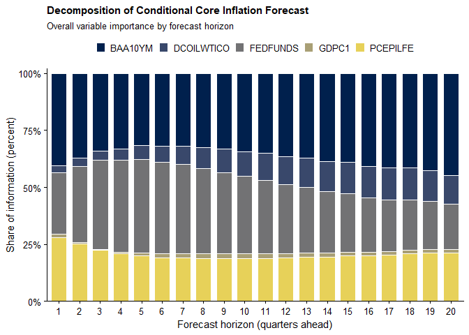
The results below are based on the overall variable importance measure, which quantifies the total contribution of each variable to the forecast, taking into account both historical observations and future conditioning constraints.
It is evident that he importance of the credit spread increases steadily with the forecast horizon. This pattern suggests that financial conditions—particularly corporate credit risk—play an increasingly prominent role in shaping medium-term inflation dynamics. This finding is consistent with evidence that credit spreads contain predictive information for demand-side pressures (e.g., Lopez-Salido et al., 2017; Caldara and Herbst, 2019).
By contrast, oil prices contribute more modestly to the core inflation forecast. Their importance rises slightly at longer horizons—an intuitive result given that core inflation excludes energy components and oil affects inflation only indirectly through production costs and aggregate demand.
The federal funds rate, although unconstrained in the scenario, contributes through its historical values. Its importance peaks at a lag of roughly five quarters, consistent with standard estimates of monetary policy transmission (e.g., Christiano et al., 1996).
Finally, GDP growth receives minimal weight in the decomposition. This reflects its weak marginal signal once financial and commodity variables are accounted for and aligns with evidence that real activity indicators offer limited incremental predictive content for inflation (Stock and Watson, 2007).
The plot below reports the marginal variable importance:
mi_df <- v_imp$marginal_variable_importance %>%
  filter(variable %in% c("BAA10YM", "DCOILWTICO")) %>%
  group_by(horizon) %>%
  ungroup() %>%
  mutate(variable = factor(variable, levels = c("BAA10YM", "DCOILWTICO")))


p3 <- ggplot(mi_df, aes(x = factor(horizon), y = share, fill = variable)) +
  geom_col(width = 0.85) +
  scale_y_continuous(labels = label_percent(), expand = c(0, 0),
                     breaks = c(0, 0.25, 0.5, 0.75, 1.0)) +
  scale_fill_manual(values = PALETTE_VAR[c("BAA10YM", "DCOILWTICO")],
                    drop = FALSE) +
  labs(title    = "Decomposition of Conditional Core Inflation Forecast",
       subtitle = "Marginal variable importance by forecast horizon",
       x = "Forecast horizon (quarters ahead)",
       y = "Share of information (percent)") +
  theme_boi() + theme(legend.position = "top")

p3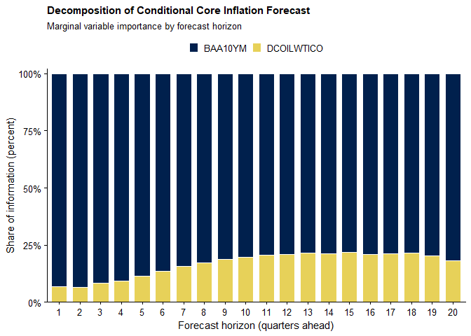
The marginal importance results broadly confirm the dominant role of the credit spread. Unlike overall importance, however, marginal importance measures the share of forecast weight attributable to future conditioning constraints. For the credit spread, this share ranges from roughly 24% to 30% across horizons, indicating that the conditional forecast is highly sensitive to the assumed future path of credit market conditions.
Taken together, the overall and marginal importance measures highlight an important distinction:
The results emphasize the dominant role of the credit spread in shaping the conditional inflation forecast and the delayed, indirect influence of oil prices.
After examining the dynamic relationships estimated by the VAR and their implications for scenario transmission, we proceed to generate a conditional forecast.
Creating a conditional forecast requires:
cond_path)cond_var)The code below illustrates the implementation:
# Construct conditioning matrix
cond_path <- cbind(baa_scen, oil_scen)

# Generate conditional forecast
fct_constr <- cforecast(
  fit,
  cond_path = cond_path,
  cond_var  = 4:5
)
The object fct_constr contains the full conditional
forecast, including the projected paths of all variables in the system
consistent with the imposed scenario.
The figure below illustrates the conditional forecast of core inflation under the assumed scenario. The imposed widening in the corporate credit spread generates a pronounced disinflationary impulse at short horizons. Within the reduced-form VAR, this shock is accompanied by an implied accommodative response of the policy rate.
The contribution of oil prices increases gradually over the forecast horizon, reflecting the indirect transmission of energy-cost shocks to core inflation through production costs and aggregate demand. By contrast, the initial spike in the credit spread produces a sharp negative effect that subsequently stabilizes at a moderate level. This pattern is consistent with the scenario design, in which spreads revert toward a slightly higher plateau rather than continuing to widen.
# Build a plotting data set for core inflation with history and both forecasts

pce_scen   <- fct_constr$forecast[, "PCEPILFE"]

t04 <- bind_rows(
  sample_data %>% transmute(date, type = "Historical", value = PCEPILFE),
  tibble(date = forecast_dates, type = "Baseline (unconditional)", value = pce_base),
  tibble(date = forecast_dates, type = "Scenario", value = pce_scen)
)

pce_hist <- sample_data %>% transmute(date, value = PCEPILFE, type = "Historical")
pce_df <- bind_rows(
  pce_hist,
  tibble(date = forecast_dates, value = pce_base,
         type = "Baseline (unconditional)"),
  tibble(date = forecast_dates, value = pce_scen, type = "Scenario"),
  tibble(date = last_date, value = tail(pce_hist$value, 1),
         type = "Baseline (unconditional)"),
  tibble(date = last_date, value = tail(pce_hist$value, 1),
         type = "Scenario")
)
p4 <- ggplot(pce_df, aes(date, value, linetype = type, group = type)) +
  geom_line(linewidth = 0.55, color = "black") +
  scale_linetype_manual(values = c("Historical" = "solid",
                                   "Baseline (unconditional)" = "dotted",
                                   "Scenario" = "dashed")) +
  scale_y_continuous(breaks = c(0.0, 0.5, 1.0)) +
  scale_x_date(breaks = as.Date(paste0(seq(1990, 2020, 10), "-01-01")),
               date_labels = "%Y") +
  labs(title = "Core Inflation Forecasts (PCE Excluding Food and Energy)",
       x = NULL, y = "Percent, quarterly rate") +
  theme_boi() + theme(legend.position = "none")

suppressWarnings(p4)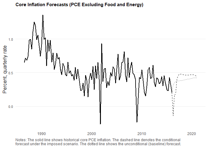
The composition of a conditional forecast can be obtained using
cforecast_composition(). The function decomposes the
scenario-induced forecast revision for a chosen target variable into
contributions from each conditioning variable.
fct_comp <- cforecast_composition(
  fct_constr,
  target_var = 2
)
To visualize the decomposition across forecast horizons:
# Add explicit horizon index
fct_comp$horizon <- 1:20

# Reshape to long format
df_long <- fct_comp %>%
  pivot_longer(
    cols      = -horizon,
    names_to  = "variable",
    values_to = "contribution"
  )

# Plot stacked contributions by horizon
ggplot(
  df_long,
  aes(x = factor(horizon),
      y = contribution,
      fill = variable)
) +
  geom_col(width = 0.8) +
  labs(
    title = "Composition of the Conditional Forecast",
    subtitle = "Contributions by variable and forecast horizon",
    x = "Forecast horizon (quarters ahead)",
    y = "Contribution to forecast",
    fill = NULL
  ) +
  scale_fill_viridis_d(option = "cividis", end = 0.9) +
  theme_classic(base_size = 12) +
  theme(
    plot.title    = element_text(face = "bold", size = 11),
    plot.subtitle = element_text(size = 10),
    axis.title    = element_text(size = 11),
    axis.text     = element_text(size = 10),
    legend.position = "top",
    legend.text     = element_text(size = 10),
    legend.key.size = unit(0.35, "cm")
  )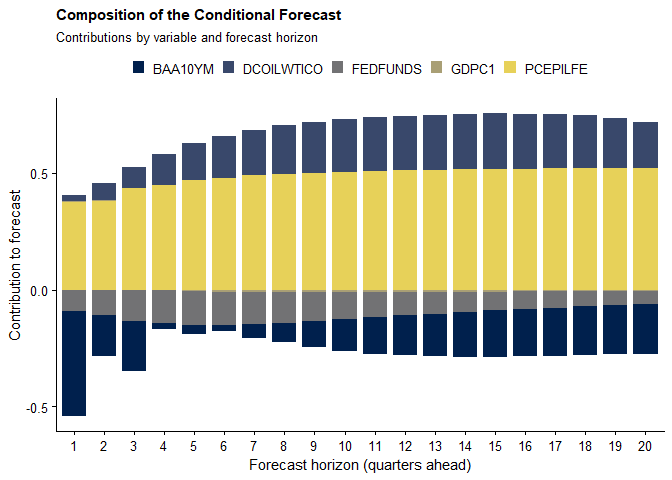
The decomposition clarifies the sources of the scenario-driven forecast revision. Although oil prices contribute visibly to the forecast composition, the variable-importance measures indicate that this effect is largely driven by the magnitude of the imposed oil-price path rather than by a strong model-implied sensitivity of core inflation to oil prices.
This distinction is economically important.
In scenarios that impose mechanically specified or stylized paths, variable-importance measures provide an ex ante indication of whether those assumptions are likely to materially affect the target forecast. More broadly, the decomposition helps discipline scenario design and interpretation by distinguishing between:
This directly informs policy communication. It identifies the pivotal elements of the narrative and highlights which imposed details are economically consequential for the variables of interest.
The views expressed here are solely of the author and do not necessarily represent the views of the Bank of Israel.
Please note that cforecast is still under development
and may contain bugs or other issues that have not yet been resolved.
While we have made every effort to ensure that the package is functional
and reliable, we cannot guarantee its performance in all situations.
We strongly advise that you regularly check for updates and install any new versions that become available, as these may contain important bug fixes and other improvements. By using this package, you acknowledge and accept that it is provided on an “as is” basis, and that we make no warranties or representations regarding its suitability for your specific needs or purposes.