The purpose of dvir is to implement state-of-the-art algorithms for DNA-based disaster victim identification (DVI). In particular, dvir performs joint identification of multiple victims.
The methodology and algorithms of dvir are described in
The dvir package is part of the pedsuite, a collection of R packages for pedigree analysis. Much of the machinery behind dvir is imported from other pedsuite packages, especially pedtools for handling pedigree data, and forrel for the calculation of likelihood ratios. A comprehensive presentation of these packages, and much more, can be found in the book Pedigree Analysis in R.
To get the current official version of dvir, install from CRAN as follows:
install.packages("dvir")Alternatively, the latest development version may be obtained from GitHub:
# install.packages("remotes")
remotes::install_github("magnusdv/dvir")library(dvir)We illustrate joint DVI analysis using a toy example from Vigeland & Egeland (2021), shown below. Three victim samples (V1, V2, V3) are to be matched against three missing persons (M1, M2, M3) from two families.
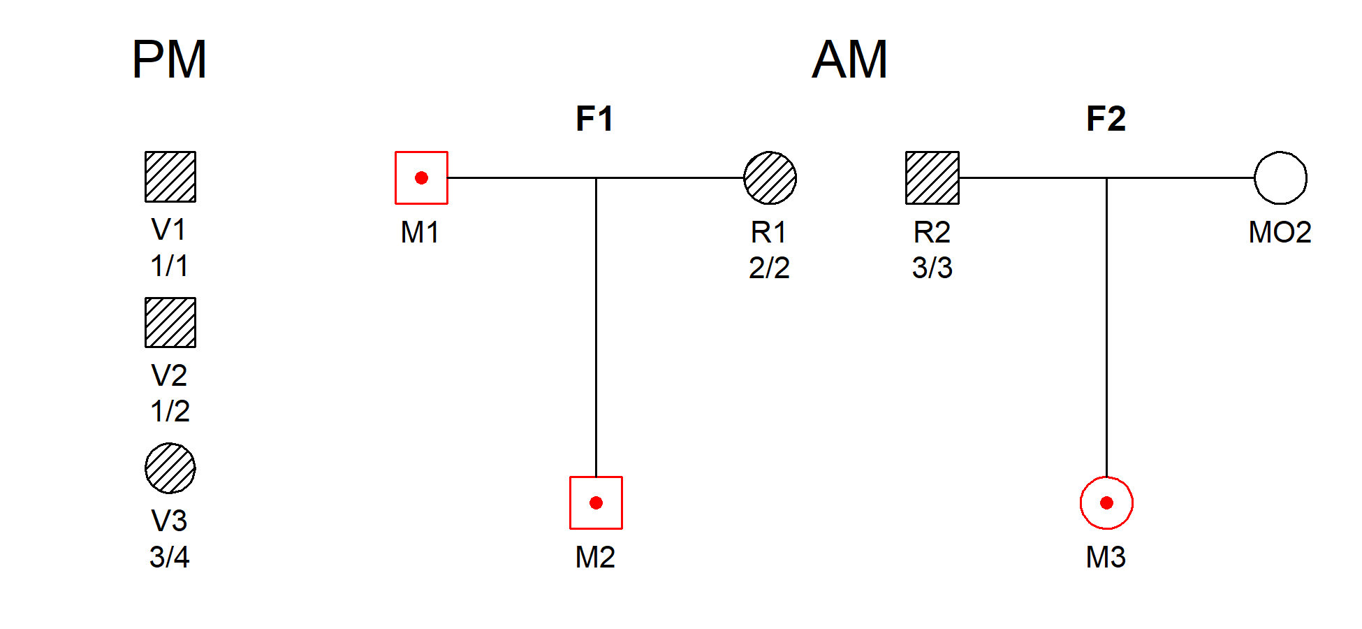
The hatched symbols indicate genotyped individuals. This simple example uses a single marker with 10 equifrequent alleles denoted 1, 2, …, 10. The observed genotypes are shown in the figure.
DNA profiles from victims are referred to as post mortem (PM) data, while the ante mortem (AM) data contain profiles from the reference individuals, R1 and R2.
The function dviJoint() performs a joint likelihood
search over all valid assignments.
joint = dviJoint(example2)
#> DVI dataset:
#>  3 victims (2M/1F): V1, V2, V3
#>  3 missing (2M/1F): M1, M2, M3
#>  2 reference individuals: R1, R2
#>  2 pedigrees: F1, F2
#> Markers: 1
#> Number of assignments: 14 (exact)
The output contains the log-likelihood of each of the 14 assignments,
and likelihood ratios (LRs) comparing the most likely solution with each
of the others. Thus the first row has LR = 1, while larger
values indicate less likely assignments:
| V1 | V2 | V3 | loglik | LR | M1 | M2 | M3 | |
|---|---|---|---|---|---|---|---|---|
| 1 | M1 | M2 | M3 | -16.118 | 1 | V1 | V2 | V3 |
| 2 | M1 | M2 | * | -17.728 | 5 | V1 | V2 | * |
| 3 | * | M2 | M3 | -18.421 | 10 | * | V2 | V3 |
| 4 | M1 | * | M3 | -20.030 | 50 | V1 | * | V3 |
| 5 | * | M1 | M3 | -20.030 | 50 | V2 | * | V3 |
| 6 | * | M2 | * | -20.030 | 50 | * | V2 | * |
| 7 | * | * | M3 | -20.030 | 50 | * | * | V3 |
| 8 | * | M1 | * | -21.640 | 250 | V2 | * | * |
| 9 | M1 | * | * | -21.640 | 250 | V1 | * | * |
| 10 | * | * | * | -21.640 | 250 | * | * | * |
| 11 | M2 | M1 | M3 | -Inf | Inf | V2 | V1 | V3 |
| 12 | M2 | M1 | * | -Inf | Inf | V2 | V1 | * |
| 13 | M2 | * | M3 | -Inf | Inf | * | V1 | V3 |
| 14 | M2 | * | * | -Inf | Inf | * | V1 | * |
The columns V1, V2 and V3 give the PM-oriented assignment: each
victim is either paired with a missing person or remains unassigned
("*"). The columns M1, M2 and M3 give the AM-oriented view
of the same assignments.
We see that the most likely joint solution is V1 = M1, V2 = M2 and V3 = M3.
For complete DVI analysis, the main function is
dviSolve(). It combines several steps, including
exclusions, undisputed identifications, pairwise LR calculations, joint
analysis of unresolved families, and conclusions based on generalised
likelihood ratios (GLRs).
We illustrate this with the built-in dataset fire, which
includes three victim samples and three missing persons from the same
family. The function plotDVI() gives an overview:
plotDVI(fire, style = 2)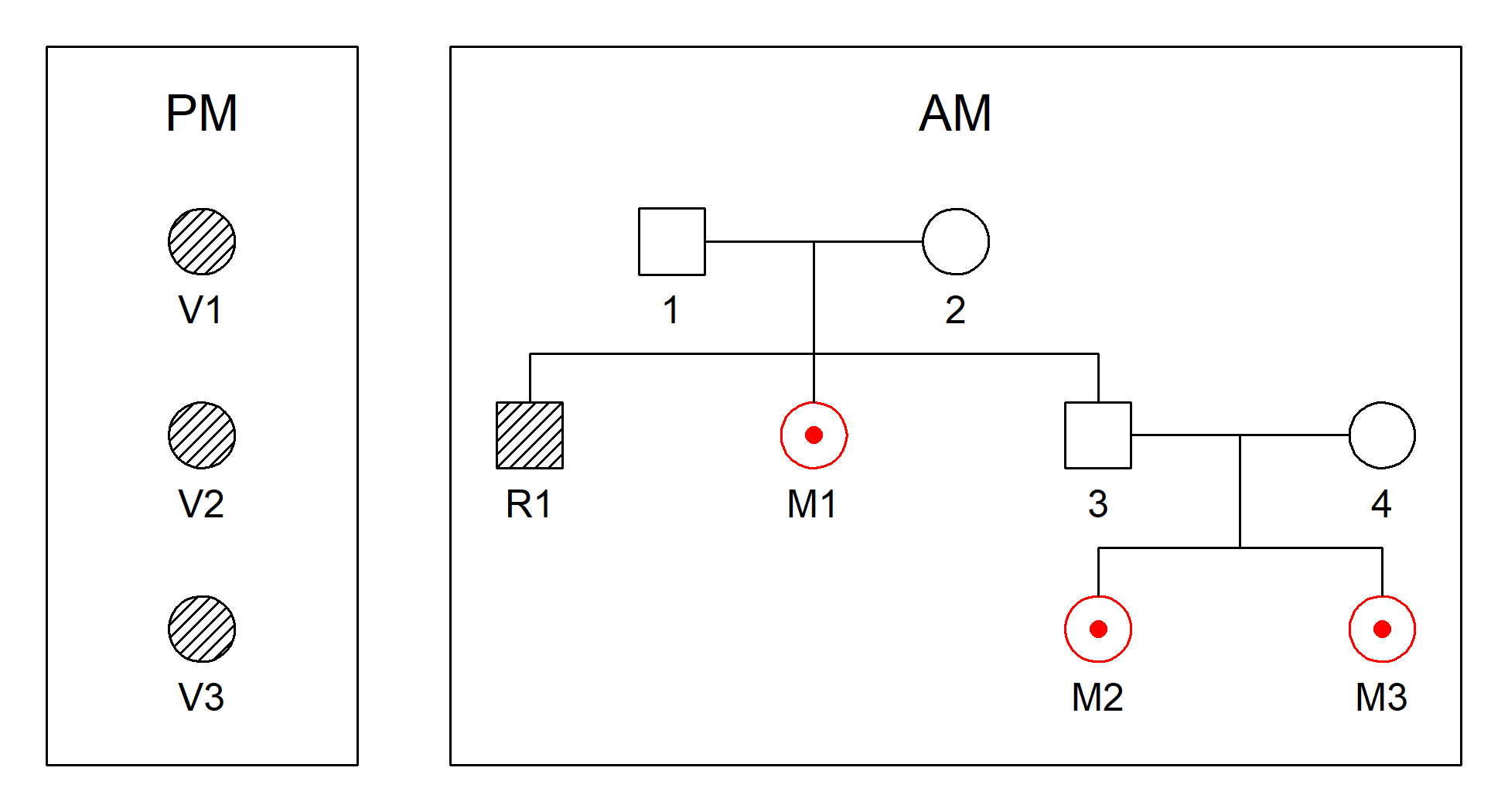
Here is the complete workflow using LR threshold 10 000:
res = dviSolve(fire, detailedOutput = TRUE, threshold = 1e4, verbose = TRUE)
#>
#> ------ Checking dataset  [+0.0s | 0.0s] ----------
#>
#> Ok
#>
#> ------ Nonidentifiable MPs  [+0.0s | 0.0s] -------
#>
#> None
#>
#> ------ Exclusions, iteration 1  [+0.0s | 0.0s] ---
#>
#> No exclusions
#>
#> ------ Undisputed, iteration 1  [+0.0s | 0.0s] ---
#>
#> No change; breaking loop
#>
#> ------ AM-driven: Simple families  [+0.1s | 0.1s]
#>
#> 0 simple families
#>
#> ------ AM-driven: Complex families  [+0.0s | 0.1s]
#>
#> 1 complex family: F1
#>
#> Number of assignments: 34 (exact)
#>
#>   Family Missing Sample       LR        GLR      Conclusion                            Comment
#> 1     F1      M1     V1 121.3476   70582.39     Match (GLR)                  Joint: {M1,M2,M3}
#> 2     F1      M2  V2/V3       NA 2947149.10 Symmetric match Full siblings: {M2, M3} = {V2, V3}
#> 3     F1      M3  V2/V3       NA 2947149.10 Symmetric match Full siblings: {M2, M3} = {V2, V3}
#>
#> ------ PM-driven: Remaining victims  [+0.2s | 0.4s]
#>
#> No remaining victims
#>
#> ------ Analysis complete  [+0.0s | 0.4s] ---------
The output contains AM-oriented and PM-oriented summary tables,
including conclusions and comments. With
detailedOutput = TRUE, the result also contains the
pairwise LR matrix, the exclusion matrix, and the joint tables used in
the analysis:
res$AM| Family | Missing | Sample | LR | GLR | Conclusion | Comment |
|---|---|---|---|---|---|---|
| F1 | M1 | V1 | 121.35 | 70582.39 | Match (GLR) | Joint: {M1,M2,M3} |
| F1 | M2 | V2/V3 | NA | 2947149.10 | Symmetric match | Full siblings: {M2, M3} = {V2, V3} |
| F1 | M3 | V2/V3 | NA | 2947149.10 | Symmetric match | Full siblings: {M2, M3} = {V2, V3} |
res$PM| Sample | Missing | Family | LR | GLR | Conclusion | Comment |
|---|---|---|---|---|---|---|
| V1 | M1 | F1 | 121.35 | 70582.39 | Match (GLR) | Joint: {M1,M2,M3} |
| V2 | M2/M3 | F1 | 36.56 | 2947149.10 | Symmetric match | Full siblings: {V2, V3} = {M2, M3} |
| V3 | M2/M3 | F1 | 1.31 | 2947149.10 | Symmetric match | Full siblings: {V2, V3} = {M2, M3} |
res$LRmatrix| M1 | M2 | M3 | |
|---|---|---|---|
| V1 | 121.348 | 398.582 | 398.582 |
| V2 | 0.583 | 36.564 | 36.564 |
| V3 | 0.002 | 1.312 | 1.312 |
res$exclusionMatrix| M1 | M2 | M3 | |
|---|---|---|---|
| V1 | 0 | 0 | 0 |
| V2 | 0 | 0 | 0 |
| V3 | 0 | 0 | 0 |
res$jointTables
(truncated)| V1 | V2 | V3 | loglik | LR | M1 | M2 | M3 |
|---|---|---|---|---|---|---|---|
| M1 | M2 | M3 | -257.73 | 1.00 | V1 | V2 | V3 |
| M1 | M3 | M2 | -257.73 | 1.00 | V1 | V3 | V2 |
| * | M2 | M3 | -268.90 | 70582.39 | * | V2 | V3 |
| * | M3 | M2 | -268.90 | 70582.39 | * | V3 | V2 |
| M2 | M1 | M3 | -272.63 | 2947149.10 | V2 | V1 | V3 |
| M3 | M1 | M2 | -272.63 | 2947149.10 | V2 | V3 | V1 |
In the fire example, V1 is identified as M1 by joint GLR
analysis (Egeland & Vigeland, 2025). The two remaining victims are
matched to the two missing full siblings M2 and M3, but the data do not
distinguish between the two sibling assignments. This is reported as a
symmetric match.