![]()
shadowVIMP is an R package for variable selection that
reduces the number of covariates in a statistically rigorous and
informed way, identifying the most informative predictors. This package
implements a method that performs statistical tests on the Variable
Importance Measures (VIMP) obtained from the Random Forest (RF)
algorithm to determine whether each covariate is statistically
significant and truly informative. In contrast to widely used methods,
such as selecting the top n covariates with the highest VIMP or
choosing covariates with a VIMP above a certain threshold, the method
implemented in shadowVIMP allows for a statistical
justification of whether a given VIMP is sufficiently large to be
unlikely due to chance. The main function of the package,
shadow_vimp(), outputs a table indicating whether each
covariate is informative, along with its associated (adjusted) p-values.
In addition, the plot_vimps() function provides a
convenient way to visualise the VIMPs obtained from the algorithm,
including unadjusted, FDR- and FWER-adjusted p-values. Details on the
method, a realistic example of its usage, and guidance on interpreting
the results can be found in the vignette:
vignette("shadowVIMP-vignette").
The shadowVIMP package can be installed in the following
way::
install.packages("shadowVIMP")Imagine you are working with a dataset with many variables and you want to select the subset of the most informative covariates. Instead of computing the variable importance, displaying it on variable importance plots, and (somewhat arbitrarily) selecting the set of informative features, you can use the method implemented in this package and select the subset of features in a more robust way. The following example shows the basic use case.
library(shadowVIMP)
library(magrittr)
library(ggplot2)

data(mtcars)

# For reproducibility
set.seed(789)
# Value of num.threads parameter
global_num_threads <- 1

# Standard usage
# WARNING 1: When working with real data, increase the value of the niters parameter or leave it at the default value.
# WARNING 2: To avoid potential issues with using multiple threads on CRAN, we set num.threads to 1, by default it is set to half of the available threads, which speeds up computation.
vimp_seq <- shadow_vimp(data = mtcars, outcome_var = "vs", niters = c(30, 100, 150), num.threads = global_num_threads)
#> alpha  0.3
#> 2025-06-05 10:25:11: dataframe = mtcars niters = 30 num.trees = 10000. Running step 1
#> Variables remaining:  10
#> alpha  0.1
#> 2025-06-05 10:25:22: dataframe = mtcars niters = 100 num.trees = 10000. Running step 1
#> 2025-06-05 10:25:37: dataframe = mtcars niters = 100 num.trees = 10000. Running step 50
#> 2025-06-05 10:25:53: dataframe = mtcars niters = 100 num.trees = 10000. Running step 100
#> Variables remaining:  9
#> alpha  0.05
#> 2025-06-05 10:25:54: dataframe = mtcars niters = 150 num.trees = 10000. Running step 1
#> 2025-06-05 10:26:07: dataframe = mtcars niters = 150 num.trees = 10000. Running step 50
#> 2025-06-05 10:26:22: dataframe = mtcars niters = 150 num.trees = 10000. Running step 100
#> 2025-06-05 10:26:37: dataframe = mtcars niters = 150 num.trees = 10000. Running step 150
#> Variables remaining:  7

# Summary of the results
vimp_seq
#> shadowVIMP Result
#>
#> Call:
#>  shadow_vimp(niters = c(30, 100, 150), data = mtcars, outcome_var = "vs", num.threads = global_num_threads)
#>
#>    Step Alpha Retained Covariates
#>  Step 1  0.30                  10
#>  Step 2  0.10                   9
#>  Step 3  0.05                   7
#>
#> Count of significant covariates from step 3 per p-value correction method using the pooled approach
#>  Type-1 Confirmed FDR Confirmed FWER Confirmed
#>                 7             7              6

# Print informative covariates according to the pooled criterion (with and without p-value correction)
vimp_seq$final_dec_pooled
#>   varname      p_unadj   p_adj_FDR  p_adj_FWER Type1_confirmed FDR_confirmed
#> 1     cyl 0.0007401925 0.002467308 0.007401925               1             1
#> 2    qsec 0.0007401925 0.002467308 0.007401925               1             1
#> 3     mpg 0.0014803849 0.002467308 0.011843079               1             1
#> 4    disp 0.0014803849 0.002467308 0.011843079               1             1
#> 5      hp 0.0014803849 0.002467308 0.011843079               1             1
#> 6    carb 0.0014803849 0.002467308 0.011843079               1             1
#> 7      wt 0.0177646188 0.025378027 0.071058475               1             1
#> 8    drat 0.0747594375 0.093449297 0.224278312               0             0
#> 9    gear 0.0969652110 0.107739123 0.224278312               0             0
#>   FWER_confirmed
#> 1              1
#> 2              1
#> 3              1
#> 4              1
#> 5              1
#> 6              1
#> 7              0
#> 8              0
#> 9              0

# The significance level used in each step of the procedure:
vimp_seq$alpha
#> [1] 0.30 0.10 0.05

# Were all covariates deemed insignificant at any step of the pre-selection? If so, which step?
# If `step_all_covariates_removed == 0`, then at least one covariate survived the pre-selection
vimp_seq$step_all_covariates_removed
#> [1] 0

# Check the time needed to execute each step of the algorithm and the entire procedure
vimp_seq$time_elapsed
#> $step_1
#> [1] 0.181146
#>
#> $step_2
#> [1] 0.5276175
#>
#> $step_3
#> [1] 0.7348017
#>
#> $total_time_mins
#> [1] 1.443565

# Check the call code that was used to create the inspected object
vimp_seq$call
#> shadow_vimp(niters = c(30, 100, 150), data = mtcars, outcome_var = "vs",
#>     num.threads = global_num_threads)

# Check the VIMPs of the covariates and their shadows from the last step of the procedure
vimp_seq$vimp_history %>% head()
#>        mpg      cyl     disp       hp     qsec     carb       wt      drat
#> 1 32.96580 37.83467 34.28494 44.40825 69.39776 24.06262 15.92240  6.592342
#> 2 33.94531 37.67475 33.80626 43.52956 69.47350 22.87792 15.14960 11.407349
#> 3 30.08375 37.37923 35.83397 45.54814 63.48126 21.02905 19.53125  9.903495
#> 4 32.87286 37.27228 33.33198 44.62708 66.72462 21.53476 16.72543 12.559785
#> 5 33.31543 37.87766 35.51419 46.53287 68.73776 23.26442 16.94575 11.323333
#> 6 32.14069 37.56510 34.74886 45.31037 67.73211 22.76118 17.46005 10.717524
#>       gear mpg_permuted cyl_permuted disp_permuted hp_permuted qsec_permuted
#> 1 5.764364    -6.069204  -3.32899537    -8.1562793    7.681771     16.844710
#> 2 4.598629     4.078202   2.89716983    13.9188568   18.325314     -4.697359
#> 3 6.940662    -3.242185   2.70553361     4.3478057   -1.002965     -3.033623
#> 4 8.191079     8.515609  -0.06092051     0.2708662   -5.778261      2.359071
#> 5 7.602294    -5.753136   0.34546070    -4.3777628    3.339719     16.449674
#> 6 7.541206    -5.267411  -0.50446983    -4.0950592   -1.733074     -5.538990
#>   carb_permuted wt_permuted drat_permuted gear_permuted
#> 1    -3.2699946   -6.661017     -2.508818     3.3687412
#> 2    -2.8813075   -1.537203     -8.378585    -1.6538532
#> 3    -4.7045122    9.585241     28.771112     7.1048423
#> 4    11.3272227    2.210888      1.430094    -2.1331894
#> 5     0.8828882   -6.429090     -4.002469     0.4812786
#> 6     0.1989782   -6.730972     -6.458763    -2.7823118

# Inspect in detail two steps of pre-selection
#  vimp_seq$pre_selection$step_1
#  vimp_seq$pre_selection$step_2
You can visualize your results in the following way:
plot_vimps(
  shadow_vimp_out = vimp_seq,
  text_size = 10,
  legend.text = element_text(size = 40),
  axis.text = element_text(size = 30)
) +
  patchwork::plot_annotation(
    title = "shadowVIMP Results",
  ) &
  theme(plot.title = element_text(size = 45, face = "bold"))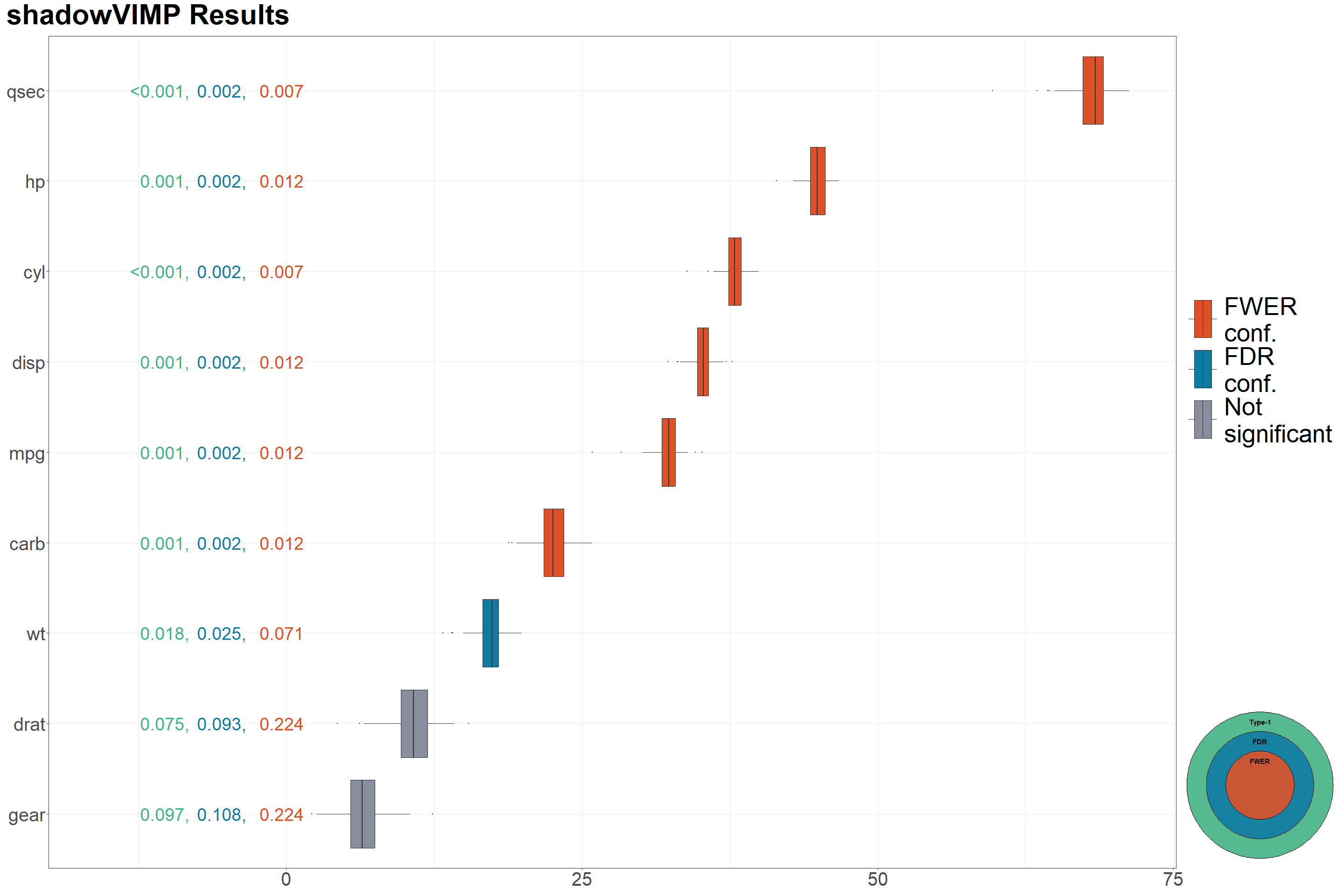
For a more realistic and detailed example of how to use this package,
and the theory behind the method, see
vignette("shadowVIMP-vignette").
If you encounter a clear bug, please file an issue with a minimal reproducible example.